In any case each parameter key and value needs enclosure in two double quotes,i.e. “Key” and “Value”. In .uds files

Basic parameterization

|| ParameterList || *(ss) || Parameter, Value

CAEnsembleSize

How many automaton domains should be devised. By default the domains are of equal size and become listed into an automaton pool from which the processes pick and execute sequentially the domains.

The random number generator assures the domains to become differently initialized. This is because each process has a different seed.

XMAX

Determines a global recrystallized volume fraction at which the simulation is stopped, the results postprocessed and the program exits.

TIMEMAX

Serves to stop the simulation as does XMAX control but when a simulated realtime (not program execution time!), is reached.

Anyhow, the simulation does not simulate growth farther in time than the maximum annealing time provided.

NMAX

Controls the stopping of the simulation after a certain number of integration steps.

CellSize

Reads in as micrometer, defines the edge length, and thus the discretization of the cubic voxel.

It should be scaled such that even the smallest grain of interest is represented by a sphere equivalent radius of at least 10 cells.

Cells smaller than 100 nanometer certainly are no longer in accordance with a mesoscopic model at the micron-scale.

3DCAEdgeLengthInCellsRD

3DCAEdgeLengthInCellsND

3DCAEdgeLengthInCellsTD

Defines the voxelization of each automaton domain, while RD is parallel to x, ND parallel to y, and TD to z, currently limited to 1600 as uint32 is utilized to store the unique assignment of cells and grains

MeanDefGrainSizeinRD

MeanDefGrainSizeinND

MeanDefGrainSizeinTD

Reads in micron, only of significance when DefStructureSynthesis is “1”

DefStructureSynthesis

Determines which deformation microstructure synthesis model is desired. “1” renders a grid of equally-sized cuboid grains should be constructed, “2” constructs discrete Poisson-Voronoi.

In order to avoid bias, the tessellation is sampled at random from a much larger continuous realization of a Poisson point process.

MeanDefSizePoissonDiameter

Reads in micron, only of significance when DefStructureSynthesis is “2”

NucleationDensityLocalCSR

Assuming each domain maps a random point process, how many nuclei would on average be observed in the domain.

CSRNucleation

Allows the placement of bulk nuclei inside the domain when set to either “1” or “2”.

“1” enforces always the same number of nuclei in each automaton which are placed in space according to random 3D coordinates.

“2” enforces that the domain itself is perceived as framing a much larger Poisson point process from which all points that fall in the domain are taken and mapped on the voxel grid.

Mind that “1” and “2” sample slightly different, though uncorrelated point processes. For domains of EdgeLengthInCells sizes larger 1000 spatial correlations of the PRNG become an issue. If in doubt test and utilize the MersenneTwister.

GBNucleation

Allows the placement of nuclei at boundaries among deformed grains when set to either “1” or “2”.

“1” enforces nuclei at all boundaries regardless the disorientation of the two adjoining grains.

“2” enforces nucleation at discrete grain boundaries only to occurr at high-angle boundaries, assuming a default threshold disorientation of 15degree

GBNucDensity2Number

GBNucRhoDiff2Density

Currently heuristic grain boundary nucleation rate modeling parameter.

GBNucMaximumScatter

Controls how strongly are grain boundary nuclei at most deviating from the matrix orientation.

IncubationTimeModel

“1” assumes nucleation to occur and grow at t=0seconds, i.e. instantaneously/site-saturated.

“2” assumes nuclei to start growing after a delay, the probability distribution of the delay times is a Rayleigh distribution.

IncubationTimeScatter Scales in seconds the only parameter of the Rayleigh distribution according to which the nuclei become placed.

Mobility model

Determines as to how the grain boundary mobility is parameterized from a disorientation among two grains.

“1” follows the approach taken by Sebald and Gottstein to leave boundaries separating less than 15deg as practical immobile,

all others of equal mobility and only to provide the close to 40deg about 111 disorientations in misorientation space an higher value (“GS”)

“2” adopts an approach going back to Humphreys and Huang that low-angle grain boundaries are practical immobile only up to a disorientation of several degrees after which a smooth sigmoidal shape is assumed.

At the moment in this model 2, close to 40°<111> boundaries are not specifically more mobile than other high-angle grain boundaries.

Output flags

RenderingOfMicrostructure

“0” no microstructure snapshot is outputted, further speeds up the simulation because minimizing file interaction

“2” 2D zsections of the RDND plane are outputted taken at TD = 0.5, reliable option when the structure evolution is to be judged qualitatively, as one would section in SEM/EBSD

“3” 3D binary files are written with MPI I/O that store the voxelized microstructure. Mind color model and hint on how to import into visualization environment.

RenderingColorModel

Defines the coloring model of the rendering as this allows directly the RGB triplets to be read into visualization software

“1” disjoint grains with unsigned int IDs

“2” IPFZ coloring with aka inverse polefigure coloring.

Please mind that the details (white point location, RGB gradients) differ from vendor to vendor.

For details consider the code and mind the possibility of stretching the RGB gradient asymmetrically over the standard triangle.

RenderingBoundaries

Allows to identify all voxel located at a boundary among deformed grains to be plot when set to “1”.

As with generating 3D raw data, these options should be omitted whenever possible to reduce file interaction, MPI I/O is utilized.

OutputLogBoundaries

If set to “1” a file detailing all connected voxel the form a discrete grain boundary patch are outputted with properties of the adjointing grains.

OutputSingleGrainStats

When set to “1” renders for each automaton a detailed history of how all grains have evolved to study impingement topologies and growth concurrencies.

OutputOfHPF

Calculate host grain distance function as detailed in the model description that can be found in the reference section.

OutputRXFrontStats

Developers option: when set to “1” all CA! output detailed loginformation on the status of their interface cell list.

This can help to find minimal sized container lengths in order to optimize further program performance and to reduce the dynamic memory footprint.

The basic idea of the automaton is that it accumulates a linear container of interface cells and runs two managing list that store positions

in this container that can be written to safely or which have recrystallized strongly enough to infect new cells. These lists are maintained throughout each simulation step.

The purpose of this list management is to minimize re-allocations and to maximize spatial and temporal locality in the cache lines.

Most microstructure paths S_V(X) tend to have a two-fold characteristic in the way that at the beginning of the transformation when

growth dominates more cells infect neighbors than already recrystallized cells become decommissioned for recycling.

At some point however the area of the RX front that is this umimpinged to grow reduces progressively while at the same time more and more cells become decommissioned/switched off.

Working on a linear array to which always fragments are appended this renders a progressively stronger and fragmented list containing gaps the activity check of which creates unnecessary overhead.

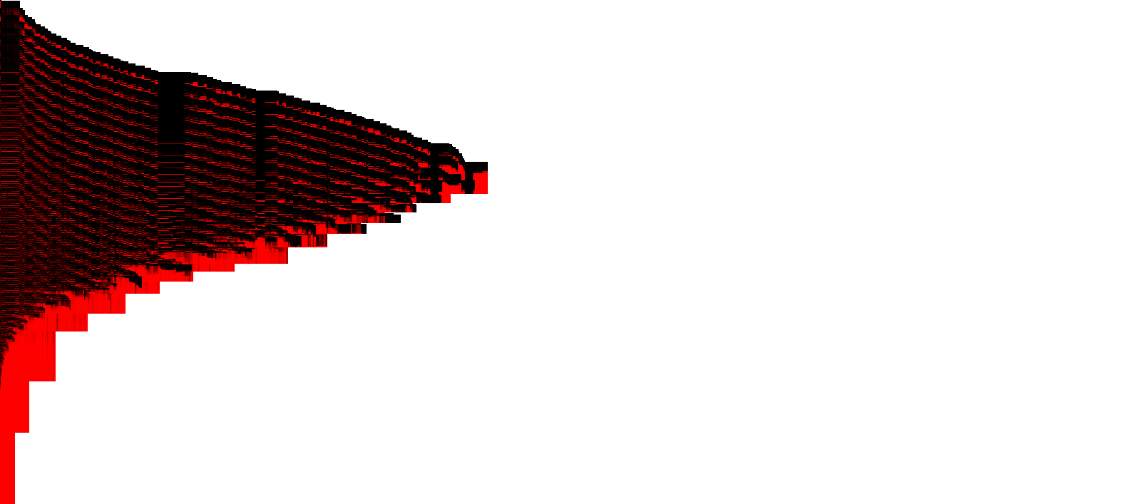
Mind the defragmentation option to reduce these gaps and as well the developer functionality FRAGMENTATION RADAR which when defined active in the code #define FRAGMENTATION_RADAR

generates a 2D graph that elucidates the occupancy of the cell array suggesting room for further improvement.

A fragmentation radar is read like a book from the upper left corner to the lower right.

Each pixel in each horizontal line represents a the average number of active cells in a block of cells BLOCKLENGTH.

Red denotes low activity (fragmented) while black is optimal.

Each vertikal lines denotes one simulation step.

Integrator and performance

|| IntegratorAccuracy || *(ss) || Parameter, Value

MAXFILLPERSTEP

Controls the volume increment that the fastest migrating boundary protrudes into a cell. Reducing this value from the default “0.1” renders simulations slower,

as the number of integration steps scales approximately linear. When increased up to its maximum 0.5 cuts integration accuracy.

RediscretizationSteps

Controls into how many equi-sized time steps the interval [0,tmax] becomes rediscretized.

InitialCacheSizeRXCells

How many of all cells in the network should be preallocated to become at some point active in the front.

For finely discretized automata with even the smallest grains 5-10 cells in spherical equivalent radius values between 0.1-0.2 are sensible defaults.

The OutputRXFrontStats can provide information on how to reduce further this number, in any case however, the automaton reallocates memory cells, if permitted by the operating system, but at the cost of execution speed.

ReCacheSizeRXCells

Controls with how many elements the cell container is extended when more cells become active then expected. In such case, the smaller ReCacheSiteRXCells the more potential small reallocations.

Material properties

|| MaterialProperties || *(ss) || Parameter, Value

ZeroKelvinShearModulusG0

Reads in Pascal, mind at zero Kelvin!

FirstOrderdG0dT

Reads in Pascal, linear shear modulus temperature coefficient

ZeroCelsiusBurgersVector

Reads in meter, mind at zero degree Celsius!

AlloyConstantThermalExpCoeff

FirstOrderThermalExpCoeff

SecondOrderThermalExpCoeff

Thermal lattice expansion coefficients appearing in Willey’s model, C constants see Hatch JE, Aluminum, see also Touloukian.

MeltingTemperature

Reads in degrees Celsius!

Grain boundary migration

LAGBm0

Reads in m^4/Js, Preexponential factor intrinsic mobility of low-angle boundaries, default truncation at 15degrees disorientation among adjoining grains

LAGBHact

Reads in eV, activation enthalpy low-angle grain boundaries

HAGBm0

HAGBHact

GSm0

GSHact

Corresponding values for general high-angle grain boundaries, and those special GS boundaries close to 40deg111 in misorientation space

RHModelHAGBm0

Reads in m^4/Js, preexponential factor intrinsic mobility of high-angle boundaries

RHModelHAGBHact

Reads in eV, activation enthalpy high-angle grain boundaries

RHModelLAGBHAGBCut

RHModelLAGBHAGBTrans

RHModelLAGBHAGBExponent

parameterizes sigmoidal model “2” as m0 * exp(-Hact/kT)* (1.0 - Cut exp(- Trans (DisoriAngle/Trans)^ Exponent)

Recovery modelling

|| RecoveryParameter || *(ss) || Parameter, Value

Mind that the following properties have not yet been fully validated!

RecoveryConsider

allow for a gradual reduction of the dislocation density to mimic a reduction of the stored energy, choose the rate determin step

“1” Erik Nes’s lateral jog drift controlled thermally activated glide aka vacancy diffusion controlled

“2” Erik Nes’s solute diffusion aka drag controlled network growth approach

All other numbers, no recovery

RecoveryVacancyDiffGeometry

Vacancy core diffusion model parameter

RecoveryVacancyDiffPreexp

Vacancy core diffusion preexponential

RecoveryVacancyDiffHact

eV, Vacancy core diffusion activation enthalpy

RecoverySoluteDiffPreexp

Solute drag diffusion model preexponential

RecoverySoluteDiffHact

eV, Solute drag diffusion activation enthalpy

RecoverySoluteLsPropFactor

Solute drag solute pinning point distance proportionality factor

RecoverySoluteConcentration

Solute drag solute concentration

RecoveryParameterAlpha3

Nes model alpha3 constant

RecoveryParameterKappa2

Nes model jog separation kappa2 constant

RecoveryParameterC3

Nes model C3 parameter

RecoveryParameterC4

Nes model C4 parameter

RecoveryParameterC5

Nes model C5 parameter

following:

Nes, E.

Recovery Revisited

Acta Metallurgica et Materialia, 1995, 43, 2189-2207

http://dx.doi.org/doi:10.1016/0956-7151(94)00409-9

Particle drag modelling

|| ZenerDragParameter || *(ss) || Parameter, Value

ZenerConsider

Should the classical Zener-Smith drag relation be utilized to simulate slowed grain boundary migration

“0” no

“1” drag is constant for all boundaries in the whole domain, then the dispersion is taken from the first line in EvoDraggingParticles

“2” drag is time-dependent in accord with the particle dispersion evolution detailed in EvoDraggingParticles

ZenerAlpha

Prefactor appearing in the various geometric limiting cases, classically 3/2

ZenerGamma

Grain boundary energy 0.324 J/m^2 from Meyers Murr Interfacial

Texture components

|| IdealComponents || *(sffff) || Name, IdealcomponentBunge1, IdealcomponentBunge2, IdealcomponentBunge3, IntegrationRange

Here typical modal orientations that are often identified with Euler space symmetry positions or orientations which show strong maxima in experimental ODFs aka Standardlagen are listed. Each orientation in the simulation is categorized to the closest of all these idealcomponents. Is an orientation not included in the integration range specified of any component, it is considered random/phon.

Microstructure snapshots

|| RenderMicrostructure || *(sf) || Local recrystallized fraction, local value

Add one line for each automaton-local recrystallized fraction at which microstructure snapshots (either 2D or 3D) should be taken. The format is “X” 0.1, i.e. to render at ten percent recrystallized.

|| RenderOnlyTheseRegions || *(i) || CAID indices start from 0 to n minus one

List all CA IDs [0, CAEnsembleSize-1] that should be included in the plotting. This option allows to reduce drastical the amount of snapshots taken and helps reducing file system congestion.

Annealing profile T(t)

|| ProcessingSchedule || *(ff) || time, temperature linearized heating profiles

For numerical performance it is admissible to coarsen the linearization of measured heating profiles rather than to import thousands of points.

Deformed grains pool

|| DeformedGrainsPool || *(ffffff) || Bunge e1, Bunge e2, Bunge e3, rho0, dsubav0, disoriav0

By default the deformed grain pool provides a list of grains all of which can but not necessarily are required of all properties different. Random sampling from this list and placing on sequentially on a 3D grid generates spatially uncorrelated MODF. Mind that a departure from the well-known MacKenzie misorientation distribution is per se not a sign of spatial correlation in the case of a non-random ODF, as the MacKenzie distribution is inferred from a random texture!

for the interested reader:

Mason, J. K., Schuh, C. A.

The generalized Mackenzie distribution: Disorientation angle distributions for arbitrary textures

Acta Materialia, 57, 2007, 4186-4197

http://dx.doi.org/doi:10.1016/j.actamat.2009.05.016

Recrystallized grains pool

|| RXGrainsPool || *(ffff) || Bunge e1, Bunge e2, Bunge e3, tincub

By default this is the current way of devising in a flexible manner many different recrystallization nuclei.

Further settings

|| HeuristicRXFrontListDefragmentation || *(sf) || Recrystallized fraction, local value

This option allows to defragment the cell container by copying explicitly pieces of information from cells far apart from the start of the container to the gap formed by cells which have become decommissioned, i.e. INACTIVE. This allows in the subsequent time steps to reduce the total number of cells that have to be checked, and hence increases performance and cache-locality. Experience has provided sensitive defaults.

|| EvoDraggingParticles || *(ff) || time, fr

Can be utilized to prescribe the Zener drag by a priori Zener drag simulations. Please mind that strictly speaking when Zener drag affects significantly microstructure transformation it occurs often concurrently to RX which is when such concept cannot be applied.

|| SingleGrainVolOverTime || *(sf) || Recrystallized fraction, local value

Controls at which automaton-local recrystallized fraction the size of the grains should be measured and stored in main memory such that it can later serve to interpolate the grain size during postprocessing.